Species Observations Explorer

Biodiversity databases make temporally and spatially extensive primary biodiversity data (i.e. species observations) available to a wide range of users. However, because of the intrinsic nature of most of the observations (e.g. opportunistic or non-systematic and presence-only), biodiversity datasets have considerable limitations including: sampling bias in favour of recorder distribution, lack of assessment of sampling effort, and lack of coverage of the distribution of all organisms. This interactive application maps where, and for which taxonomic groups, there are enough species observations for ecological analyses in applied or theoretical contexts. It reports of the quality of the data that goes beyond the data abundance, to inform you about the sampling effort and the relevance of lack of data.

ABSENCE OF SPECIES OR ABSENCE OF OBSERVERS?

Species Observation Explorer uses the half-ignorance algorithm [1] to map the bias and lack of sampling effort inherent to the species observations, henceforth called Ignorance. This approach represents the data into a scale 0 to 1 (0 being a theoretical absolute credibility in the data and 1 being absolute ignorance). With the algorithm settings you decide at how many observations the lack of data for a species is equally likely due to absence of the species as to absence of observers (i.e. I = 0.5, defined by O_0.5). Any further data in a cell builds up the trust in the data (i.e. real absences of species).

The rationale assumes that species groups share similar bias. Observations are reported by people with varied field skills and accuracy. However, observers are assumed to be fond of or specialist on one or more taxonomic groups (e.g. families, orders or even classes), rather than on individual species. Hence it is appropriate to use species’ groups as a surrogate for sampling effort (henceforth, a reference taxonomic group or RTG). It is straightforward to assume that the lack of reports of any species from the RTG e.g. birds is likely due to a lack of ornithologists, rather than to the total absence of birds. The inverse logic also holds true. That is, the larger the number of observations of species from the RTG in a grid cell, the more likely it is that absence of a particular species reflects a true absence.

This dynamic application allows you to explore any RTG at any spatial and temporal resolution. Currently, it accesses data stored in the Global Biodiversity Information Facility (GBIF), but it allows filtering by institutions that provide data to GBIF.

You can read more about Ignorance Scores here.

HOW TO USE IT

On the first tab “Map” you can explore the spatial bias of the selected reference taxonomic group, in the selected time frame (“Search Options“). On the map you will see in a scale of white-green the density of the data for the selected RTG. Beware that this is ALL the data that is available, but YOUR search will filter observations in terms of e.g. time window and Basis of Record. Unfiltered data is only shown to give you an idea of the presence and density of observations, and is not a quality report. Also, this hexagons have not the same area in the Equator than towards the poles. Your selected data and its quality will show only after you have finished your search, and the green density map will be toggled off.

To perform a search, do like this:

1. Draw a polygon using any of the shape-buttons  on the top-left. If you chose the rectangle-shape you can click in one corner and then drag it out to appropriate size, using the pentagram-shape you can determine the shape yourself by creating points/vertices on each click with the mouse.
2. On the panel to the left there are three tabs. The first one is called “Grid Options“. There you can choose the width of the grid cells. If you want your grid to cover the full extent of your selected study area check the “Buffer” check-box. If you want squared grid cells, uncheck the “Hexagonal grid” check-box. In this case, the grid follow the map projection and all cells will have the same (ground) area, no matter where in the map.
3. Choose your Reference Taxonomic Group from the list. The groups shown in the lists are common taxas, but you can override this option in the tab (“Search Options“) (see below).
4. Click the “Grid” button  (on the “Grid Options” tab). Don’t you like it? Change the options and click “Grid” again.
5. Do you like the grid? Click the “Search” button .
6. Now you can see the ignorance in each grid cell.
   
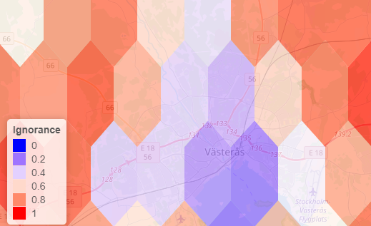
   Note that elongated grid cells towards the Poles are due to the map projection, but all have the same ground area.
7. You can allways start over by clicking on “Clear” .
8. Under “Ignorance Scores Assumptions” you specify how many observations you think is appropriate to define O_0.5, the number of observations required per grid cell to decrease the ignorance to 0.5.
   You can calculate ignorance over “Raw Observations” (using the O_0.5RTG), “Observation Indices” (i.e. the average number of observations per observed species; using the O_0.5 per species), or you can choose the “Combined” ignorance score, that uses both parameters.
9. More search options are available under the “Search Options” tab.
   1. Specifying a taxonomic ID will override the selected RTG. You will need to know the taxonomic ID to use this option, this can be found at the GBIF Taxonomic Backbone.
   2. You can select the time frame (years) of observations to be included by dragging the two start-stop points, data from 1900 to the current year are available (although the bar goes up to 2020).
   3. The basis of records to be included can be determined, e.g. if you do not want to include fossil specimen. Select more classes using the Shift + Ctrl/Cmd keys. Selecting none, selects all.
   4. Also the country of observation, publishing country and publishing organization can be chosen. In the special case of Publishing Organization you will be able to chose among the 100 most commonly looked for organizations. If you don’t find the one you are looking for, you can enter the UUID of the organization you wish. For example, ArtDatabanken-Sweden UUID is b8323864-602a-4a7d-9127-bb903054e97d, GBIF-Sweden UUID is 4c415e40-1e21-11de-9e40-a0d6ecebb8bf. For more UUIDs, check here.
10. When you have changed any search parameters, click the “Search” button again to see the new result.
11. Finally, after the search is performed, you can download the grid (.SHP file) and the data table (as .CSV file) by clicking the “Download” button  on the “Download” tab. At present, there are only a few Coordinate Reference Systems to choose from, but more are coming on demand. Files will be compressed in a .TAR file (for compatibility across platforms) in your default Download folder. You can open the file with 7zip.

On the second tab “Data” the data obtained for each grid cell is ploted and displayed as a table.

Author: Alejandro Ruete PhD, 2017
Greensway AB. Uppsala, Sweden.

E-mail: analys@greensway.se

[1] Ruete A. 2015. Displaying bias in sampling effort of data accessed from biodiversity databases using ignorance maps. Biodiversity Data Journal 3:e5361 (article).

Keywords: citizen-science data, open-access biodiversity database, presence-only data, primary biodiversity data, sampling effort, spatial bias, species distribution model, taxonomic bias, temporal bias